This is a very important step! Before we continue, we should divide the data into training data sets to train your model; Test data sets to evaluate model performance. It is recommended to split them into 60-70% training sets and 30-40% test sets.
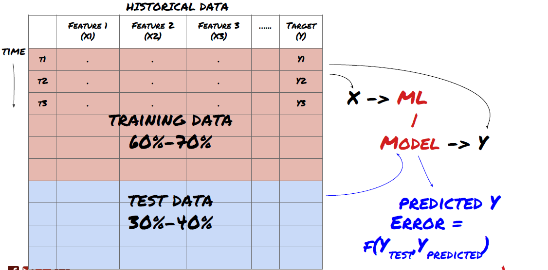
Split the data into training sets and test sets
Since training data is used to evaluate model parameters, your model may over fit these training data, and the training data may mislead model performance. If you do not retain any individual test data and use all the data for training, you will not know how well or badly your model performs on the new invisible data. This is one of the main reasons for the failure of the trained ML model in real-time data: people train all available data and are excited by the training data indicators, but the model cannot make any meaningful prediction on the untrained real-time data.
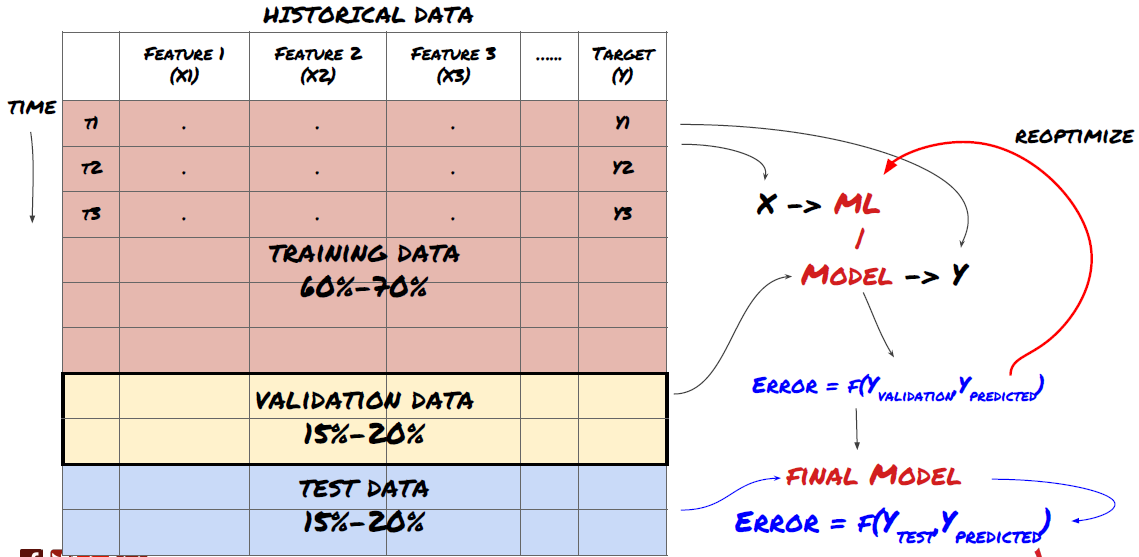
Split the data into training set, verification set and test set
There are problems with this method. If we train the training data repeatedly, evaluate the performance of the test data and optimize our model until we are satisfied with the performance, we take the test data as a part of the training data implicitly. In the end, our model may perform well on this set of training and test data, but it cannot guarantee that it can predict new data well.
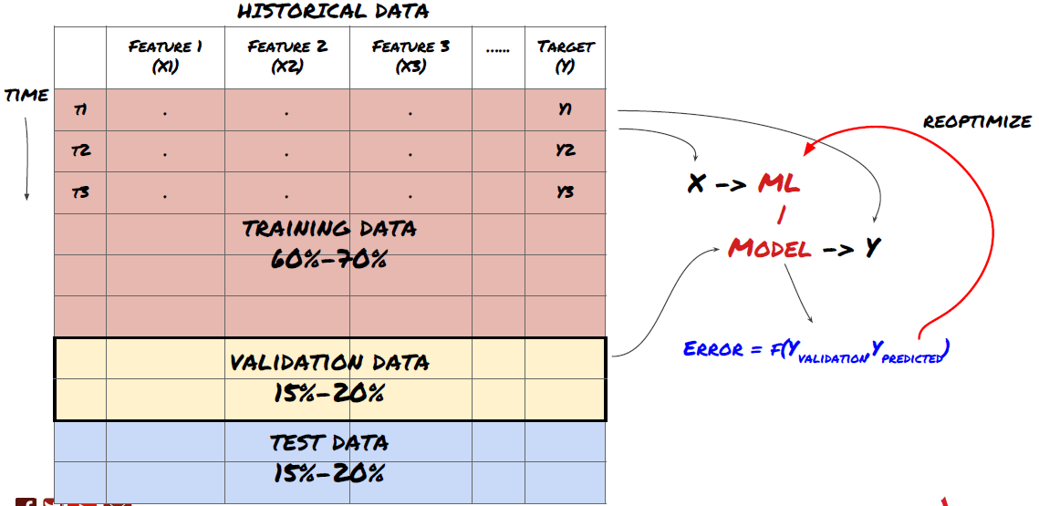
To solve this problem, we can create a separate validation dataset. Now, you can train the data, evaluate the performance of the validation data, optimize until you are satisfied with the performance, and finally test the test data. In this way, the test data will not be polluted, and we will not use any information in the test data to improve our model.
Remember, once you have checked the performance of your test data, don't go back and try to further optimize your model. If you find that your model does not give good results, discard the model completely and start again. It is suggested that 60% of training data, 20% of validation data and 20% of test data can be split.
For our question, we have three available data sets. We will use one as the training set, the second as the verification set, and the third as our test set.
# Training Data
dataSetId =  'trainingData1'
ds_training = QuantQuestDataSource(cachedFolderName=cachedFolderName,
                                    dataSetId=dataSetId,
                                    instrumentIds=instrumentIds)
training_data = loadData(ds_training)
# Validation Data
dataSetId =  'trainingData2'
ds_validation = QuantQuestDataSource(cachedFolderName=cachedFolderName,
                                    dataSetId=dataSetId,
                                    instrumentIds=instrumentIds)
validation_data = loadData(ds_validation)
# Test Data
dataSetId =  'trainingData3'
ds_test = QuantQuestDataSource(cachedFolderName=cachedFolderName,
                                    dataSetId=dataSetId,
                                    instrumentIds=instrumentIds)
out_of_sample_test_data = loadData(ds_test)
For each of these, we add the target variable Y, which is defined as the average of the next five basis values.
def prepareData(data, period):
    data['Y(Target)'] = data['basis'].rolling(period).mean().shift(-period)
    if 'FairValue' in data.columns:
        del data['FairValue']
    data.dropna(inplace=True)
period = 5
prepareData(training_data, period)
prepareData(validation_data, period)
prepareData(out_of_sample_test_data, period)Analyze data behavior and create predictive features
Now the real project construction has started. The golden rule of feature selection is that prediction ability mainly comes from features, not from models. You will find that the selection of features has a far greater impact on performance than the selection of models. Some considerations for feature selection:
Do not select a large set of features randomly without exploring the relationship with the target variable.
Little or no relationship with the target variable may lead to overfitting.
The features you select may be highly related to each other, in which case a small number of features can also explain the target.
I usually create some intuitive features, check the correlation between the target variable and these features, and the correlation between them to decide which one to use.
You can also try to perform principal component analysis (PCA) and other methods to sort candidate features according to the maximum information coefficient (MIC).
ML models tend to perform well in terms of normalization. However, normalization is difficult when dealing with time series data, because the future data range is unknown. Your data may be out of the normalization range, leading to model errors. But you can still try to force some degree of stability:
Scaling: dividing features by standard deviation or quartile range.
Centering: subtract the historical average value from the current value.
Normalization: two retrospective periods of the above (x - mean)/stdev.
Regular normalization: standardize the data into the range of - 1 to +1 and redetermine the center within the backtracking period (x-min)/(max min).
Note that since we use historical continuous average value, standard deviation, maximum or minimum values beyond the backtracking period, the normalized standardization value of the feature will represent different actual values at different times. For example, if the current value of the feature is 5 and the average value for 30 consecutive periods is 4.5, it will be converted to 0.5 after centering. After that, if the average value of 30 consecutive periods becomes 3, the value 3.5 will become 0.5. This may be the cause of the wrong model. Therefore, normalization is tricky, and you must figure out what improves the performance of the model actually (if any).
For the first iteration in our problem, we created a large number of features by using mixed parameters. Later we will try to see if we can reduce the number of features.
def difference(dataDf, period):
    return dataDf.sub(dataDf.shift(period), fill_value=0)
def ewm(dataDf, halflife):
    return dataDf.ewm(halflife=halflife, ignore_na=False,
                      min_periods=0, adjust=True).mean()
def rsi(data, period):
    data_upside = data.sub(data.shift(1), fill_value=0)
    data_downside = data_upside.copy()
    data_downside[data_upside > 0] = 0
    data_upside[data_upside < 0] = 0
    avg_upside = data_upside.rolling(period).mean()
    avg_downside = - data_downside.rolling(period).mean()
    rsi = 100 - (100 * avg_downside / (avg_downside + avg_upside))
    rsi[avg_downside == 0] = 100
    rsi[(avg_downside == 0) & (avg_upside == 0)] = 0
return rsi
def create_features(data):
    basis_X = pd.DataFrame(index = data.index, columns =  [])

    basis_X['mom3'] = difference(data['basis'],4)
    basis_X['mom5'] = difference(data['basis'],6)
    basis_X['mom10'] = difference(data['basis'],11)

    basis_X['rsi15'] = rsi(data['basis'],15)
    basis_X['rsi10'] = rsi(data['basis'],10)

    basis_X['emabasis3'] = ewm(data['basis'],3)
    basis_X['emabasis5'] = ewm(data['basis'],5)
    basis_X['emabasis7'] = ewm(data['basis'],7)
    basis_X['emabasis10'] = ewm(data['basis'],10)
    basis_X['basis'] = data['basis']
    basis_X['vwapbasis'] = data['stockVWAP']-data['futureVWAP']

    basis_X['swidth'] = data['stockTopAskPrice'] -
                        data['stockTopBidPrice']
    basis_X['fwidth'] = data['futureTopAskPrice'] -
                        data['futureTopBidPrice']

    basis_X['btopask'] = data['stockTopAskPrice'] -
                         data['futureTopAskPrice']
    basis_X['btopbid'] = data['stockTopBidPrice'] -
                         data['futureTopBidPrice']

    basis_X['totalaskvol'] = data['stockTotalAskVol'] -
                             data['futureTotalAskVol']
    basis_X['totalbidvol'] = data['stockTotalBidVol'] -
                             data['futureTotalBidVol']

    basis_X['emabasisdi7'] = basis_X['emabasis7'] -
                             basis_X['emabasis5'] +
                             basis_X['emabasis3']

    basis_X = basis_X.fillna(0)

    basis_y = data['Y(Target)']
    basis_y.dropna(inplace=True)

    print("Any null data in y: %s, X: %s"
            %(basis_y.isnull().values.any(),
             basis_X.isnull().values.any()))
    print("Length y: %s, X: %s"
            %(len(basis_y.index), len(basis_X.index)))

    return basis_X, basis_y
basis_X_train, basis_y_train = create_features(training_data)
basis_X_test, basis_y_test = create_features(validation_data)Select the appropriate statistical/ML model according to the selected questions
The choice of model depends on how the problem is formed. Are you solving supervised (each point X in the feature matrix is mapped to the target variable Y) or unsupervised learning (without a given mapping, the model tries to learn an unknown pattern)? Are you dealing with regression (forecasting the actual price in the future time) or classification (only forecasting the price direction in the future time (increase/decrease))?
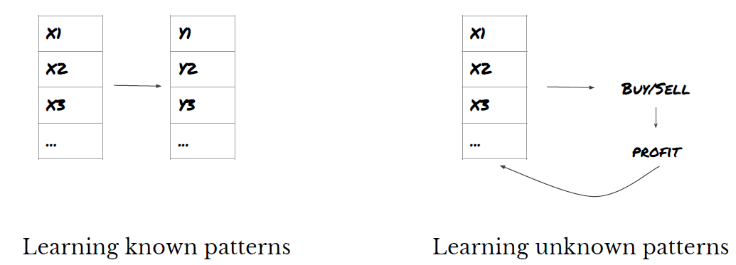
Supervised or unsupervised learning

Regression or classification
Some common supervised learning algorithms can help you get started:
Linear regression (parameters, regression)
Logistic regression (parameter, classification)
K-Nearest Neighbor (KNN) algorithm (case-based, regression)
SVM, SVR (parameters, classification and regression)
Decision tree
Decision forest
I suggest starting with a simple model, such as linear or logistic regression, and building more complex models from there as needed. It is also recommended that you read the mathematics behind the model rather than using it as a black box blindly.
Linear regression without normalization
('Coefficients: \n', array([ -1.0929e+08, 4.1621e+07, 1.4755e+07, 5.6988e+06, -5.656e+01, -6.18e-04, -8.2541e-05,4.3606e-02, -3.0647e-02, 1.8826e+07, 8.3561e-02, 3.723e-03, -6.2637e-03, 1.8826e+07, 1.8826e+07, 6.4277e-02, 5.7254e-02, 3.3435e-03, 1.6376e-02, -7.3588e-03, -8.1531e-04, -3.9095e-02, 3.1418e-02, 3.3321e-03, -1.3262e-06, -1.3433e+07, 3.5821e+07, 2.6764e+07, -8.0394e+06, -2.2388e+06, -1.7096e+07]))
Mean squared error: 0.02
Variance score: 0.96
Look at the model coefficients. We can't really compare them or say which one is important, because they all belong to different scales. Let's try normalization to make them conform to the same proportion and also enforce some smoothness.
def normalize(basis_X, basis_y, period):
    basis_X_norm = (basis_X - basis_X.rolling(period).mean())/
                    basis_X.rolling(period).std()
    basis_X_norm.dropna(inplace=True)
    basis_y_norm = (basis_y -
                    basis_X['basis'].rolling(period).mean())/
                    basis_X['basis'].rolling(period).std()
    basis_y_norm = basis_y_norm[basis_X_norm.index]

    return basis_X_norm, basis_y_norm
norm_period = 375
basis_X_norm_test, basis_y_norm_test = normalize(basis_X_test,basis_y_test, norm_period)
basis_X_norm_train, basis_y_norm_train = normalize(basis_X_train, basis_y_train, norm_period)
regr_norm, basis_y_pred = linear_regression(basis_X_norm_train, basis_y_norm_train, basis_X_norm_test, basis_y_norm_test)
basis_y_pred = basis_y_pred * basis_X_test['basis'].rolling(period).std()[basis_y_norm_test.index] + basis_X_test['basis'].rolling(period).mean()[basis_y_norm_test.index]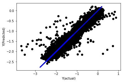
To be continued…