The inspiration of this article comes from my observation of some common warnings and traps after trying to apply machine learning technology to transaction problems during the data research on the FMZ Quant platform.
If you haven't read my previous articles, we suggest you read the automated data research environment guide and systematic method for formulating trading strategies that I established on the FMZ Quant platform before this article.
These two article addresses are here: https://www.fmz.com/digest-topic/9862 and https://www.fmz.com/digest-topic/9863.
This tutorial is intended for enthusiasts, engineers and data scientists at all skill levels. Whether you are an industry leader or a programming novice, the only skills you need are a basic understanding of Python programming language and sufficient knowledge of command line operations (being able to set up a data science project is sufficient).
The FMZ Quant platform FMZ.COM not only provides high-quality data sources for major mainstream exchanges, but also provides a set of rich API interfaces to help us carry out automatic transactions after completing data analysis. This set of interfaces includes practical tools, such as querying account information, querying high, open, low, receipt price, trading volume, and various commonly used technical analysis indicators of various mainstream exchanges. In particular, it provides strong technical support for the public API interfaces connecting major mainstream exchanges in the actual trading process.
All the above mentioned features are encapsulated into a Docker-like system. What we need to do is to purchase or lease our own cloud computing services and deploy the Docker system.
In the official name of the FMZ Quant platform, the Docker system is called the Docker system.
Please refer to my previous article on how to deploy a docker and robot: https://www.fmz.com/bbs-topic/9864.
Readers who want to purchase their own cloud computing server to deploy dockers can refer to this article: https://www.fmz.com/digest-topic/5711.
After deploying the cloud computing server and the docker system successfully, next, we will install the present largest artifact of Python: Anaconda
In order to realize all the relevant program environments (dependency libraries, version management, etc.) required in this article, the simplest way is to use Anaconda. It is a packaged Python data science ecosystem and dependency library manager.
Since we install Anaconda on the cloud service, we recommend that the cloud server install the Linux system plus the command line version of Anaconda.
For the installation method of Anaconda, please refer to the official guide of Anaconda: https://www.anaconda.com/distribution/.
If you are an experienced Python programmer and if you feel that you do not need to use Anaconda, it is no problem at all. I will assume that you do not need help when installing the necessary dependent environment. You can skip this section directly.
The final output of a trading strategy should answer the following questions:
Direction: Determine if the asset is cheap, expensive or fair value.
Opening position conditions: If the asset is cheap or expensive, you should go long or go short.
Closing position trade: if the asset is reasonably priced and we have a position in the asset (previous buy or sell), should you close the position?
Price range: the price (or range) at which the position was opened.
Quantity: the quantity of money traded (e.g., the amount of digital currency or the number of lots of commodity futures).
Machine learning can be used to answer each of these questions, but for the rest of this article, we will focus on the first question, which is the direction of the trade.
There are two types of approaches to constructing strategies: one is model-based; The other is based on data mining. These two methods are basically opposite to each other.
In the model-based strategy construction, we start from the market inefficiency model, build mathematical expressions (such as price and profit) and test their effectiveness in a long period of time. This model is usually a simplified version of a real complex model, and its long-term significance and stability need to be verified. The common trend following, mean reversion and arbitrage strategies fall into this category.
On the other hand, we look for price patterns first and try to use algorithms in data mining methods. The reasons for these patterns are not important, because only the identified patterns will continue to repeat in the future. This is a blind analysis method, and we need to check strictly to identify real patterns from random patterns. "Repeated test method", "k-line chart model" and "feature mass regression" belong to this category.
Obviously, machine learning is very easy to apply to data mining methods. Let's look at how to use machine learning to create transaction signals through data mining.
The code example uses a backtesting tool based on the FMZ Quant platform and an automated transaction API interface. After deploying the docker and installing Anaconda in the above section, you only need to install the data science analysis library we need and the famous machine learning model scikit-learn. We will not go over this section again.
pip install -U scikit-learn-Data mining
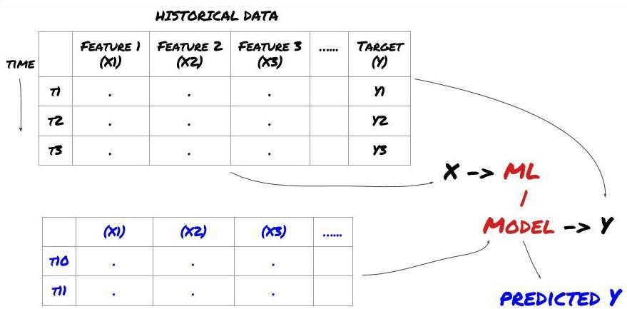
Before we begin, a standard machine learning problem system is shown in the following figure:

Machine learning problem system
The feature we are going to create must have some prediction ability (X). We want to predict the target variable (Y) and use historical data to train the ML model that can predict Y as close to the actual value as possible. Finally, we use this model to make predictions on new data where Y is unknown. This leads us to the first step:
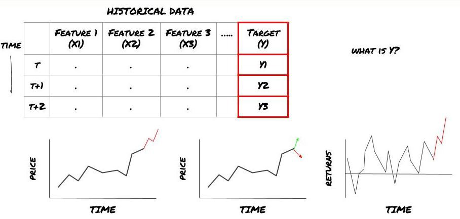
That is, in our framework above, what is Y?

What do you want to predict?
Do you want to predict future prices, future returns/Pnl, buy/sell signals, optimize portfolio allocation and try to execute transactions efficiently?
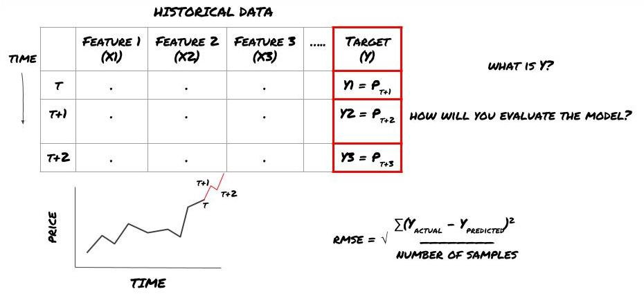
Suppose we try to forecast prices on the next timestamp. In this case, Y (t)=price (t+1). Now we can use historical data to complete our framework.
Note that Y (t) is known only in the backtest, but when we use our model, we will not know the price (t+1) of time t. We use our model to predict Y (predicted, t) and compare it with the actual value only at time t+1. This means that you cannot use Y as a feature in the prediction model.
Once we know the target Y, we can also decide how to evaluate our predictions. This is important to differentiate between the different models of the data we will try. Select an indicator to measure the efficiency of our model according to the problem we are solving. For example, if we predict prices, we can use root mean square error as an indicator. Some commonly used indicators (EMA, MACD, variance score, etc.) have been pre coded in the FMZ Quant toolbox. You can call these indicators globally through the API interface.

ML framework for predicting future prices
For demonstration purposes, we will create a prediction model to predict the expected future benchmark (basis) value of a hypothetical investment object, where:
basis = Price of Stock — Price of Future

basis(t)=S(t)−F(t)

Y(t) = future expected value of basis = Average(basis(t+1),basis(t+2),basis(t+3),basis(t+4),basis(t+5))
Since this is a regression problem, we will evaluate the model on RMSE (root mean square error). We will also use Total Pnl as the evaluation criteria.
Note: Please refer to Baidu Encyclopedia for relevant mathematical knowledge of RMSE.
Collect and clear data that can help you solve the problem at hand.
What data do you need to consider that can predict the target variable Y? If we predict the price, you can use the price data of the investment object, the trading quantity data of the investment object, the similar data of the related investment object, the index level of the investment object and other overall market indicators, and the price of other related assets.
You need to set data access permissions for these data and ensure that your data is accurate, and solve the lost data (a very common problem). At the same time, make sure that your data is impartial and fully representative of all market conditions (for example, the same number of profit and loss scenarios) to avoid bias in the model. You may also need to clean up the data to get dividends, split investment targets, continuations, etc.
If you use the FMZ Quant platform (FMZ. COM), we can access free global data from Google, Yahoo, NSE and Quandl; Depth data of domestic commodity futures such as CTP and Esunny; Data from mainstream digital currency exchanges such as Binance, OKX, Huobi and BitMex. The FMZ Quant platform also pre cleans and filters these data, such as the split of investment targets and in-depth market data, and presents them to strategy developers in a format that is easy for quantitative practitioners to understand.
To facilitate the demonstration of this article, we use the following data as the 'MQK' of the virtual investment target. We will also use a very convenient quantitative tool called Auquan's Toolbox. For more information, please refer to: https://github.com/Auquan/auquan-toolbox-python.
# Load the data
from backtester.dataSource.quant_quest_data_source import QuantQuestDataSource
cachedFolderName = '/Users/chandinijain/Auquan/qq2solver-data/historicalData/'
dataSetId = 'trainingData1'
instrumentIds = ['MQK']
ds = QuantQuestDataSource(cachedFolderName=cachedFolderName,
                                    dataSetId=dataSetId,
                                    instrumentIds=instrumentIds)
def loadData(ds):
    data = None
    for key in ds.getBookDataByFeature().keys():
        if data is None:
            data = pd.DataFrame(np.nan, index = ds.getBookDataByFeature()[key].index, columns=[])
        data[key] = ds.getBookDataByFeature()[key]
    data['Stock Price'] =  ds.getBookDataByFeature()['stockTopBidPrice'] + ds.getBookDataByFeature()['stockTopAskPrice'] / 2.0
    data['Future Price'] = ds.getBookDataByFeature()['futureTopBidPrice'] + ds.getBookDataByFeature()['futureTopAskPrice'] / 2.0
    data['Y(Target)'] = ds.getBookDataByFeature()['basis'].shift(-5)
    del data['benchmark_score']
    del data['FairValue']
    return data
data = loadData(ds)
With the above code, Auquan's Toolbox has downloaded and loaded the data into the data frame dictionary. We now need to prepare the data in the format we like. The function ds.getBookDataByFeature() returns the dictionary of data frames, one for each feature. We create new data frames for stocks with all characteristics.
To be continued…